Climograph

Climograph for Prescott, Arizona

http://cals.arizona.edu/watershedsteward/resources/module/Climate/climate-trends_pg8.htm

To determine the climate of a region one must study the relationship between temperature and precipitation. Climograph's plot this relationship at monthly intervals over the course of a years time. The climograph above represents the data collected from Prescott, Arizona with precipitation measured in inches and temperature in Fahrenheit. This climograph uses a red line graph in combination with a blue bar graph to show the data collected from Prescott, Arizona. The highest temperature for the year was 73 F in the month of July and the greatest amount of precipitation was recorded in the month of August at 3.5 inches.  

Similarity Matrix

http://spie.org/x48704.xml?pf=true&ArticleID=x48704

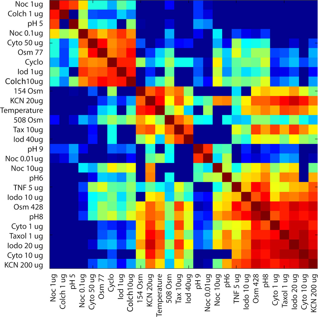
A similarity matrix is a perfect tool to use when comparing the similarity between several data points. Each square within the matrix shows the relationship between two of the data points. This similarity matrix depicts the changes that occur to the motion of tumor cells in response to drug administration. As you can see from the diagram there is a diagonal form that shows groups with similar responses.

Star Plot

http://alumni.media.mit.edu/~tpminka/courses/36-350.2001/lectures/day38/

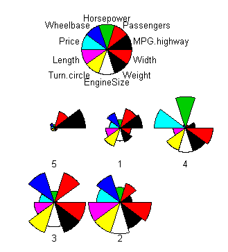
Star plots are a type of geovisualization that enable someone to compare multivariate data using variables and observations. Each star portrays a single observation. The variables that are being compared are plotted on the radii which displays each ones distinct characteristics. The length of the radii is proportional to the intensity of the variable for that data point compared with the maximum intensity of the variable across all of the data points. Star plots are often used to determine which observations are the most similar or if there are any irrelevant observations. The more correlated the variables are the closer they are together on the star plot.The plot above incorporates the star plots of 5 types of cars starting from 1, midsize, luxury, minivan, sporty, and compact. The 10 variables used for this star plot consist of: horse power, passengers, wheel base, MPG highway, width, weight, engine size, turn circle, length, and price.  From reading the star plot we are able to deduce that compact car (#5) can fit a few but not too many passengers and has great gas mileage but is not up to par with the rest of the vehicle types in every other category. Star plots would be very useful in comparing these variables while out car shopping.

Parallel Coordinate Plot

http://www.sci.utah.edu/~kpotter/Library/Papers/ge:2009:EUPC/

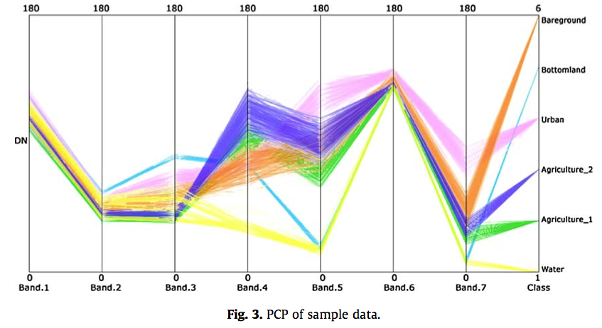
A parallel coordinate plot uses a vertical axis to plot the variables within a set or sets of data. Each set of data is plotted with connected points, with one on each axis. A parallel coordinate plot can be beneficial when attempting to apply and analyze multidimensional graphical data. The plot above uses this technique "highlight the distribution of probability values of different land cover types for each pixel, and also reflect the status of pixels with different degrees of uncertainty." The data collected in the Yellow River Delta, Shandong Province, China from different types of land cover include bare ground, bottomland, urban, agriculture 1 and 2, and water.

Histogram

http://www.ec.gc.ca/mbc-com/default.asp?lang=En&n=DEE0C80B-1

A histogram like the graph shown above presents the frequency of occurrence within a set of data.  This histogram displays the number of Greater Snow Geese at Cap Tourmente NWA for the fall of 2013. The dates range from September 13 - October 31 and number of birds seen per day varies from a little more than 5500 - a little more than 55,000. You can assess from the graph there is an extreme variation in the frequency of birds at this location over such a short period of time.

Box Plot

http://weatherstories.ssec.wisc.edu/stories/armistice_day/climate.html

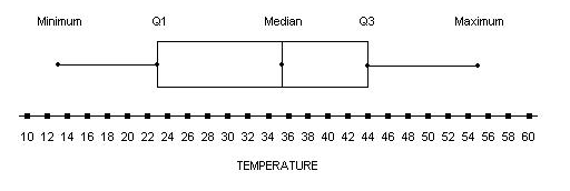
A box plot or a box and whisker diagram like the one shown above summarizes the distribution of a set of data using the median, minimum extreme, maximum extreme, and quartiles. The box plot comes in very handy when needing to compare multiple sets of data. The graph above is depicting the daily mean temperature in degrees Fahrenheit (F) for the month of November 1940, in Madison, Wisconsin. By using the box plot to display the data it is easy to gather the data off of the graph. The minimum extreme temperature for the month was a chilling 13 F, 23 F for quartile 1, 44 F for quartile 3, a median of 35.5 F, and a maximum temperature of 55 F. 

Stem and Leaf Plot

http://www.eduplace.com/math/mhm/5/06a/

The stem-and-leaf plot splits the data value into two categories, the stem for the first digit and the leaf for the last. These types of plots are frequently used for calculating averages for test results. The stem-and-leaf plot shown above is used in determining the age range for attendance at a family reunion. The ages start at 1 and go all the way up to 81. There is an eighty year difference between the age of the youngest attendee and the oldest. There is not a certain age that attended more than the others. the ages were scattered.